相関係数関係

[Take0] テスト用データの読み込み

【書式】

【コード】

import pandas as pd

df=pd.read_csv("/content/drive/MyDrive/Python_2024/002/test3.csv",encoding="Shift-JIS",index_col=0)

print(df)

【結果】

理科 国語

数学

94 80 100

90 88 85

95 70 90

90 62 95

85 86 80

80 70 80

75 79 75

70 65 65

60 75 65

60 67 60

50 75 55

50 68 45

48 60 45

ありがちな、テストの点数の表。

[Take1] 散布図を描く

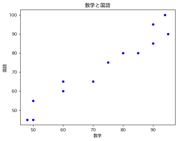
【書式】

df.plot.scatter(x=x値リスト, y=yのリスト, color="色")

【コード】

%matplotlib inline

import matplotlib.pyplot as plt

import japanize_matplotlib

import seaborn as sns

import pandas as pd

　

df=pd.read_csv("/content/drive/MyDrive/Python_2024/002/test3.csv",encoding="Shift-JIS")

　

df.plot.scatter(x="数学",y="理科",color="b")

plt.title("数学と理科")

plt.show()

　

df.plot.scatter(x="数学",y="国語",color="b")

plt.title("数学と国語")

plt.show()

【結果】

[Take2] データの相関係数を求める

【書式】

df.corr()[横のリスト][縦のリスト]

【コード】

%matplotlib inline

import pandas as pd

　

df=pd.read_csv("/content/drive/MyDrive/Python_2024/002/test3.csv",encoding="Shift-JIS")

　

print("数学と理科",df.corr()["数学"]["理科"])

print("数学と国語",df.corr()["数学"]["国語"])

【結果】

数学と理科 0.4134661925183854

数学と国語 0.9688434503857297

補足）相関係数の計算

相関係数＝偏差の積の合計÷各列の偏差平方和の積の平方根

[Take3] データの相関行列を求める

【書式】

df.corr()

【コード】

%matplotlib inline

import pandas as pd

　

df=pd.read_csv("/content/drive/MyDrive/Python_2024/002/test3.csv",encoding="Shift-JIS")

　

print(df.corr())

【結果】

数学 理科 国語

数学 1.000000 0.413466 0.968843

理科 0.413466 1.000000 0.394252

国語 0.968843 0.394252 1.000000

[Take3-1] 相関行列をヒートマップで表示する

【書式】

ライブラリ：pandas,matplotlib,seaborn

書式

sns.heatmap(df.corr()) plt.show()

【コード】

%matplotlib inline

import pandas as pd

import matplotlib.pyplot as plt

import japanize_matplotlib

import seaborn as sns

　

df=pd.read_csv("/content/drive/MyDrive/Python_2024/002/test3.csv",encoding="Shift-JIS")

　

sns.heatmap(df.corr())

plt.show()

【結果】

[Take3-2] 相関行列を散布図行列で表示する

【書式】

ライブラリ：pandas,matplotlib,seaborn

書式

sns.pairplot(data=df)

plt.show()

オプション

kind="reg" : 回帰曲線を追記する

【コード】

%matplotlib inline

import pandas as pd

import matplotlib.pyplot as plt

import japanize_matplotlib

import seaborn as sns

　

df=pd.read_csv("/content/drive/MyDrive/Python_2024/002/test3.csv",encoding="Shift-JIS")

　

sns.pairplot(data=df,kind="reg")

plt.show()

【結果】

補足）対角部分はヒストグラム

[Take4] 回帰曲線を描画する

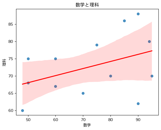
【書式】

ライブラリ：pandas,matplotlib,seaborn

書式

sns.regplot(data=df,x="横の列名",y="縦の列名",line_kws={"color":"色"}}

plt.show()

【コード】

%matplotlib inline

import matplotlib.pyplot as plt

import japanize_matplotlib

import seaborn as sns

import pandas as pd

　

df=pd.read_csv("/content/drive/MyDrive/Python_2024/002/test3.csv",encoding="Shift-JIS")

　

sns.regplot(data=df,x="数学",y="理科",line_kws={"color":"red"})

plt.title("数学と理科")

plt.show()

【結果】

[Take5] さらにヒストグラムを付け足す

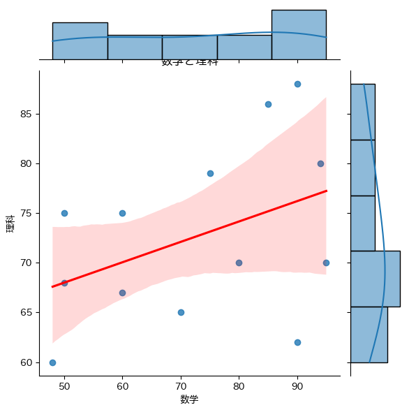
【書式】

ライブラリ：pandas,matplotlib,seaborn

書式

sns.jointplot(data=df,x="横の列名",y="縦の列名",kind="reg",line_kws={"color":"色"}}

plt.show()

【コード】

%matplotlib inline

import matplotlib.pyplot as plt

import japanize_matplotlib

import seaborn as sns

import pandas as pd

　

df=pd.read_csv("/content/drive/MyDrive/Python_2024/002/test3.csv",encoding="Shift-JIS")

　

sns.jointplot(data=df,x="数学",y="理科",kind="reg",line_kws={"color":"red"})

plt.title("数学と理科")

plt.show()

【結果】